Colorectal Cancer Proteomics
Tumour versus healthy, protein by protein.
An analysis of CPTAC proteomic data comparing colorectal tumours with healthy colon tissue. Starting from 54 samples and more than ten thousand proteins, I cleaned, filtered, imputed and normalised the data, tested every protein for a difference between the two groups, and wrote up each decision in a report.
The data
Fifty-four samples, cleaned first.
The dataset holds 21 healthy and 33 tumour samples from CPTAC, run across six TMT batches. Before anything else I removed 69 contaminant proteins, mapped every sample column to Normal or Tumour, and checked that the two groups were mixed across all six batches, so condition and batch aren't fully confounded.
- Contaminants such as keratins and trypsin removed, leaving 10,225 proteins
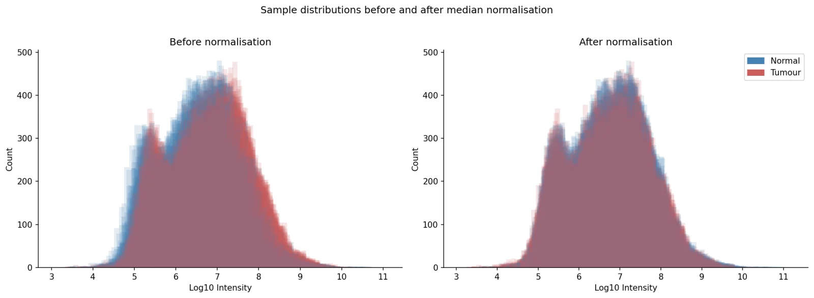
- Sample medians varied 3.4-fold, so each sample was median-normalised
- After normalisation, all 54 medians lined up at 5,836,685
Missing values
Missing, but not at random.
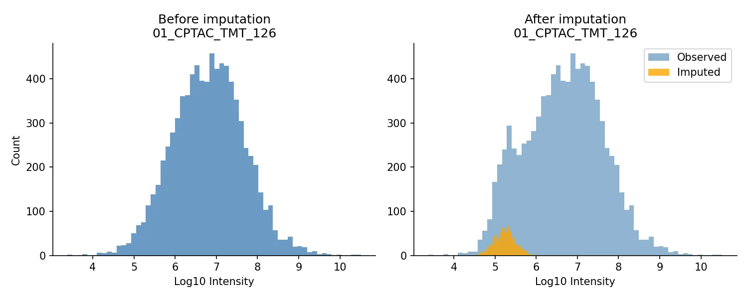
Proteins at low abundance fall below the detection limit, so an empty value usually means a small one. About 20% of values were missing per sample. I dropped proteins missing from more than 75% of samples, leaving 9,140, and filled the remaining gaps with draws from a downshifted distribution, the method Perseus uses.
- A stricter 50% cutoff could have thrown out proteins present in only one group, which may be real biology
- Dropping every protein with a gap would have left 6,366, biased towards the most abundant
- Imputed values sit in the lower tail of each sample's distribution
Testing
589 proteins changed.
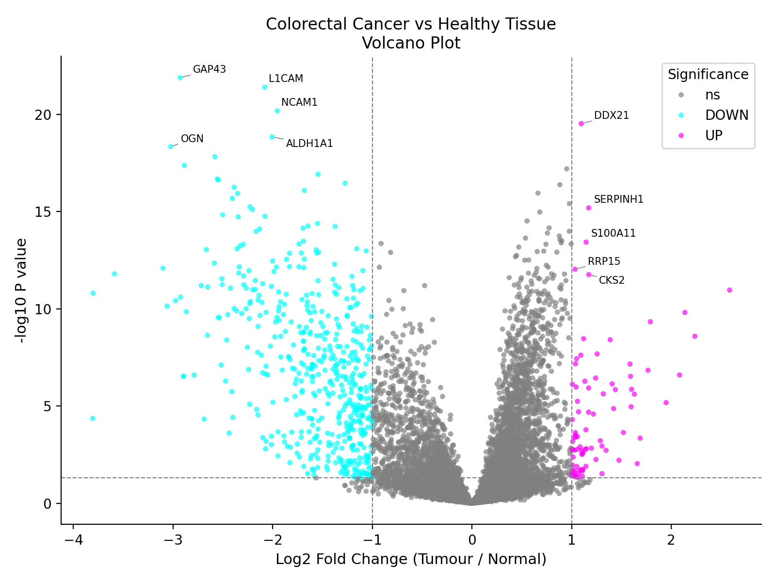
Each of the 9,140 proteins was tested with Welch's t-test on log2 intensities, 21 healthy samples against 33 tumour. A protein counted as significant only if it changed at least twofold and had p below 0.05. That gave 83 proteins up in tumour and 506 down, a pattern consistent with tumours losing the identity of normal colon tissue.
- Welch's test, because the groups differ in size and likely in variance
- Log2, because raw intensities are roughly log-normal
- With Benjamini-Hochberg correction, 544 of the 589 still passed at q ≤ 0.05
Proteins of interest
Ten proteins, up close.
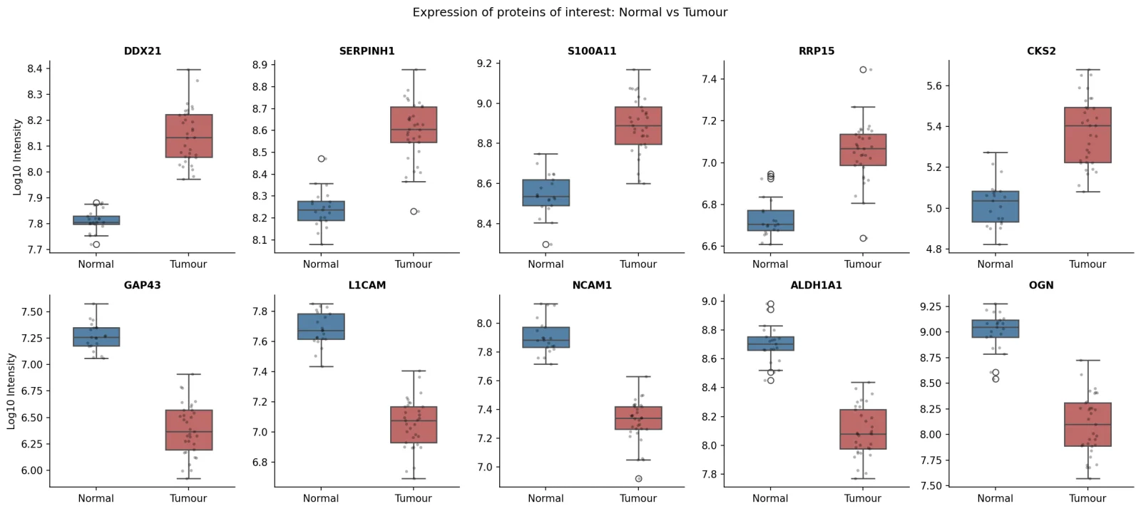
I shortlisted the five most significant proteins in each direction. Those up in tumour fit active growth: DDX21 and RRP15 support ribosome biogenesis, SERPINH1 points to matrix remodelling, and S100A11 and CKS2 both have documented links to colorectal cancer. Those down, GAP43, L1CAM, NCAM1, ALDH1A1 and OGN, fit a loss of normal colon tissue identity.
And the details.
- 54samples: 21 healthy, 33 tumour
- 9,140proteins tested after filtering
- 589changed significantly: 83 up, 506 down
Six TMT batches
01_CPTAC to 06_CPTAC, with healthy and tumour samples in every batch.
Contaminants first
69 entries tagged #CONTAM removed before any other step.
Normalisation, chosen
Median normalisation over quantile, which would force every sample into the same shape.
A fix along the way
The t-test first ran on raw intensities. On log2, DDX21's p-value went from 8.9e-14 to 3.0e-20.
Readable labels
Gene names on the volcano plot placed with adjustText so they don't overlap.
What's next
A paired test for patients who gave both tissues, and pathway enrichment across all 589 proteins.
How it's built
Python, Pandas, NumPy.
The analysis is written in Python: pandas and NumPy for the tables, SciPy for the statistics, and Seaborn and Matplotlib for every figure. The report walks through each step, the alternatives I considered and what changed along the way.
- Python
- Pandas
- NumPy
- SciPy
- Seaborn
- Matplotlib
- Proteomics
Downshifted imputation
For each sample on the log10 scale, missing values are drawn from a normal distribution centred 1.8 SD below the mean with a width of 0.3 SD, then transformed back.
Two thresholds, not one
Requiring both a twofold change and p < 0.05 avoids calling tiny effects with small p-values, or large changes built on noisy measurements.
Checking the calls
Benjamini-Hochberg correction ran as a check on the uncorrected calls: 544 of the 589 proteins still passed with the same fold-change threshold.